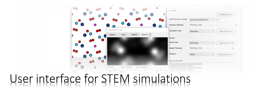
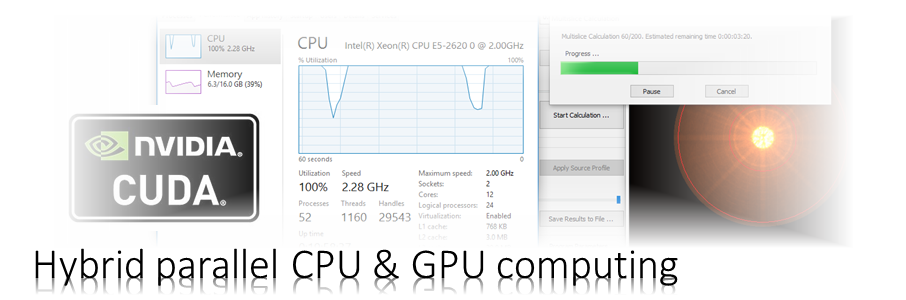
The Dr. Probe graphical user interface (GUI) provides easy access to basic STEM image simulations with direct display of results. Calculations are accelerated by using many CPU threads and your NVIDIA GPU in parallel. The software runs on 64-bit Windows operating systems.
The user interface is build in dialog form with input controls for parameter setup and managing data. Results of simulations are shown in additional data display windows.
Instrument
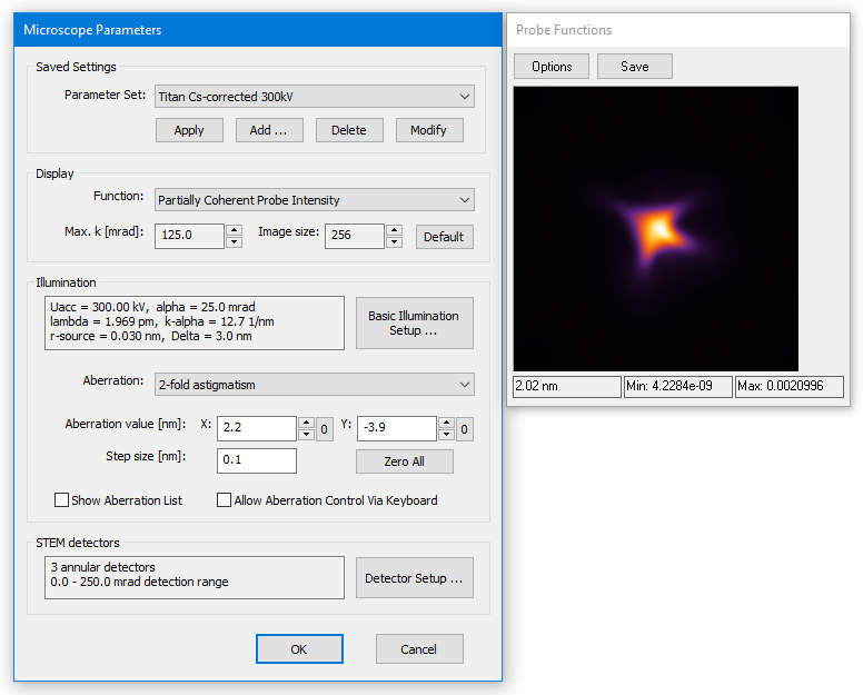
The first step of a simulation is to define parameters related the instrument. The microscope setup dialog provides controls to set and change parameters relevant for STEM image simulations. A data display window opens to the right. It reflects the current parameter setting visually with a selected type of probe function.
The dialog is organized in four sections arranged from top to bottom concerning
1. managing saved parameter settings,
2. display parameters,
3. illumination parameters, and
4. STEM detectors.
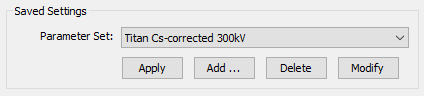
1. Presets
Saved Settings are pre-saved parameter sets related to the microscope. They allow you to quickly switch between different microscopes and specific imaging scenarios.
Select a pre-saved setting from the drop-down list and load it by pressing the [Apply] button. This will override the current settings.
Add the current settings to the lis of pre-saved settings by pressing the [Add …] button. You will be asked to specify a name for new setting. The name should be different from names of previously saved settings.
Delete the selected pre-saved setting from the list by pressing the [Delete] button.
You can also write the current parameters into an already existing pre-saved setting by pressing the [Modify] button.
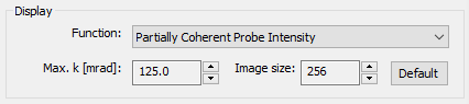
2. Display
Parameters of the probe function display are set using the display section.
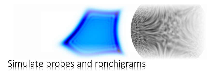
Select the active probe function to be displayed in the attached window from the dropdown list. Next to a diversity of probe functions, you can also display the aberration function and a simulated ronchigram of an artificial thin amorphous object. Each function is calculated using the current set of microscope parameters as well as with the two imaging parameters Max. k and Image size specified in the display section.
The physical sampling of the probe function is set by specifying the maximum diffraction vector k in units of milliradians. The current setting for this parameter is displayed and the number can be adjusted using the attached spin button controls. By increasing the max. diffraction vector, the image is zoomed to a finer scale for probe functions shown in real space, and to a coarser scale for functions shown in Fourier-space.
The number of image pixels used to sample the probe function in the display can be changed also with the attached spin controls.
Press the [Default] button to reset the max. diffraction vector and the image size to reasonable values for the currently selected probe function.
3. Illumination
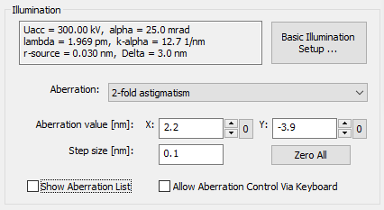
The physical parameters describing the probe formation are set in the Illumination section of the Microscope Parameters dialog.
The upper part of this section shows current values of basic illumination parameters such as:
- – the accelerating voltage Uacc,
- – the radius of the illumination aperture, i.e. the semi angle of probe convergence alpha,
- – the electron wavelength lambda,
- – the maximum incident beam vector k-alpha in the front-focal plane,
- – the effective geometric source radius (HWHM)
- – the effective defocus spread Delta
The values of these and some other parameters can be changed via an additional dialog, which opens when you press the button [Basic Illumination Setup].
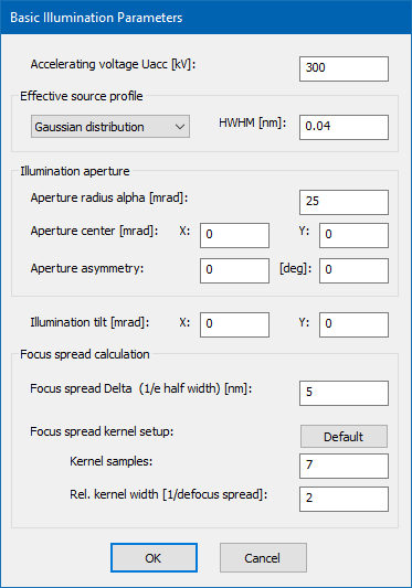
Basic Illumination Setup
Basic illumination parameters are relevant for the electron probe formation The meaning of each parameter is described separately on this page below.
The accelerating voltage Uacc of the microscope determines the kinetic energy of the probing electrons (their de Broglie wavelength) and is set here in kV units. This parameter is used in almost every part of a simulation. It is therefore one of the mots important parameters and should be checked and set beginning with a simulation.
The effective source profile limits the spatial coherence of the electron probe. A single coherent multislice calculation always considers an ideal point source. The effect of a finite source size is simulated by a later convolution of the STEM image with a respective source distribution function.
A set of source distributions is supported, including a Gaussian distribution, a Lorentz distribution, and a uniform disk shape. The source shape can be selected from the dropdown list. By selecting the ideal point source, partial spatial coherence is not applied in the simulation.
The size of the source distribution is set in terms of the half-width at half maximum height (HWHM) for continuous distributions, or as radius in case of a uniform disk source.
The aperture radius alpha in mrad units defines the maximum angle of beams in the incident convergent ray bundle with respect to the optics axis. The illumination half angle has influence on the effective probe size in STEM. In general, larger angles allow smaller probe diameters.
You can shift the illumination away from the optics axis by specifying a respective aperture center in mrad.
The aperture asymmetry parameters allow you to define an elliptical probe-forming aperture. The first parameter sets the strength of ellipticity relative to the mean aperture radius alpha defined above. For example a value of 0.1 means a 10% larger aperture radius along the long axis and a 10% lower radius along the short axis. The second parameter sets the orientation of the long axis with respect to the x-axis of the front focal plane.
The illumination beam tilt has a very similar effect as a shift of the illumination aperture and is also specified by two components in mrad. A beam tilt effectively shifts the probe aberration function relative to the illumination aperture.
The defocus spread accounts for partial temporal coherence of the probe. It describes a temporal and fast fluctuation of the defocus caused by fluctuations of lens currents, accelerating voltages, and electron emission energy.
The focus spread parameter Delta specifies the 1/e-half-width of a Gaussian focal distribution function. During the simulation of STEM images, several coherent calculations are performed for a certain set of defocus values and summed up with weights according to the focus spread kernel.
Using the explicit focus spread convolution involves repeated computations of the multislice algorithm for each scan position and will lead to a significantly larger computation time of STEM images. Therefore, the focus spread calculation can be switched on and off in the calculation setup dialog.
The number of focus-spread kernel samples defines the number of coherent calculations done with different defocus values for the explicit focal averaging. The calculation time will increase by a factor equal to this number compared to an image calculation neglecting the focus spread.
The relative kernel width determines the defocus range of the focus spread kernel in units of the focus spread parameter Delta. Usually values between 2 and 3 work sufficiently well.
Aberration
The lower part of the illumination section concerns the probe aberrations.
Select an aberration from the dropdown list and change its X and Y coefficients by changing the values in the respective edit controls. Type the number or use the spin-control attached to the right side of the edit box. The step size of the spin controls is set in the edit control below. All aberration values are in nanometer units. The probe function display will update each time you change a value.
Pressing the [0] buttons next to the spin controls will set the respective aberration coefficient to zero. All coefficients will be set to zero when you press the [Zero All].
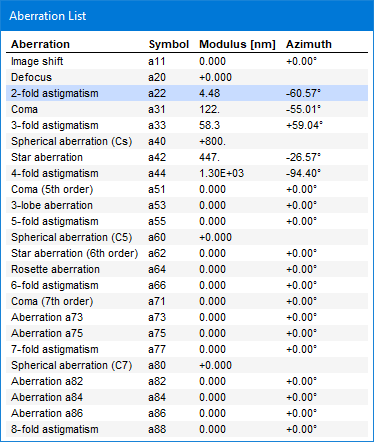
Check Show Aberration List to toggle the display of an extra window which list all aberrations and their current values in polar notation.
Clicking a row in the aberration list window will select the respective aberration as the current aberration for changing its coefficients.
The orientation of aberration coefficients as denoted by the angle in the aberration list window and by the X and Y components are with respect to the simulation axes. These axes are in general not identical to those used in aberration measurements with real microscopes. Before transferring measured aberration coefficients to the simulation, take care to adopt the values to the coordinate system used in the simulation by rotation. This task is usually non-trivial.
Check Allow Aberration Control Via Keyboard to toggle changing aberrations with the arrow keys of your keyboard. Each time you press one of the arrow keys an aberration coefficient is changed with the current step size. Left and right arrow keys change the X-coefficient. Up and down arrow keys change the Y-coefficient of the currently selected aberration. Use the page-up and page-down keys to change the current step size by a factor of ten.
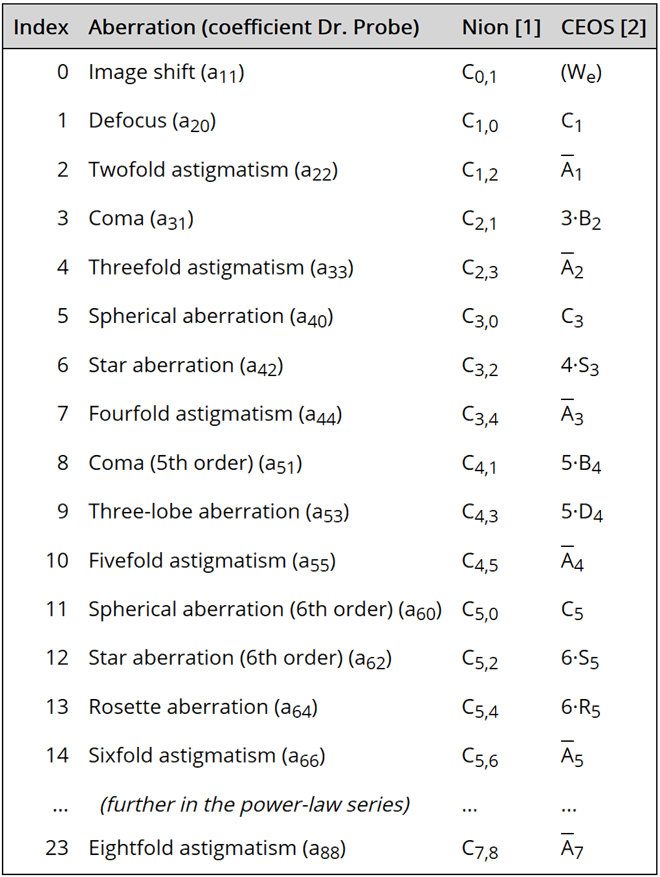
The aberration notation used by Dr. Probe is in principle identical to the notation used by NION, see Krivanek et. al (1999) [1]. For convenience, an aberration list is given below also including the relation to the notation used by CEOS, see Uhlemann & Haider (1998) [2]. Note that some aberration coefficients apply with a different magnitude compared to the CEOS notation, e.g. B2 and S3. All n-fold astigmatism coefficients have a reversed rotational sense, which is denoted by the complex conjugate of the aberration coefficient, e.g. A1, A2.
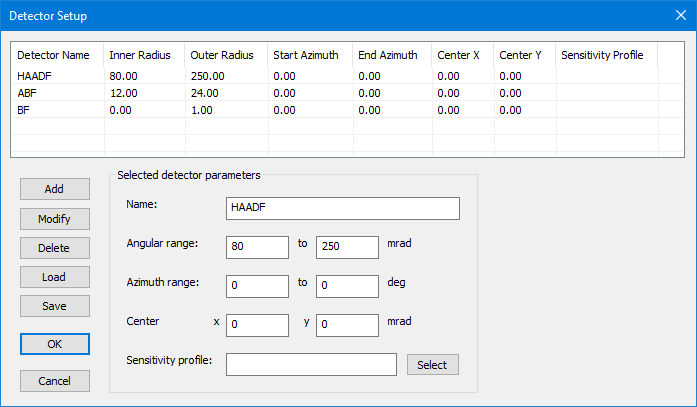
4. Detectors
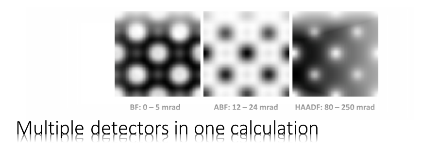
STEM detectors are defined by rings or ring segments placed the diffraction plane below the sample. Multiple detectors can be read out simultaneously in one simulation. The detector setup allows you also to specify radial sensitivity profiles to achieve even better quantitative comparisons between experiment and simulation.
Defined detectors are shown in the list with their parameters. When selecting a detector in the list, the parameters are copied to the edit controls in the lower are of the dialog.
Each detector has a unique detector name which will be used as file suffix when saving simulated STEM images to files. It is therefore recommended to use only short names such as “BF”, “ABF”, and “HAADF”.
Ring or ring segment detectors are specified by an angular range in diffraction plane, limited by an inner radius and by an outer radius in mrad units.
Ring segments require also a limited azimuth range specified in degrees measured with respect to the x axis of the simulation box. In order to prevent ambiguities, please define the azimuthal range using angles beta1 (left edit box) and beta2 (right edit box) between 0 deg and 360 deg with beta1 < beta2.
Detectors may be shifted away from the optics axis in the diffraction plane. The shift of the detector center is specified here by two parameters denoting the center coordinates (horizontal and vertical) in the diffraction plane using mrad units.
By default, the detector sensitivity is assumed to be 1, which means that the absolute square of the electron wave function os registered with 100% strength by the detector. The sensitivity of each detector can be changed by linking a file that describes a relative radial sensitivity profile. Select a file from disk by pressing the button next to the edit box or type the file name.
The detector data and the detector list content can be manipulated by the column of buttons on the lower left side of the dialog.
By pressing the [Add] button, a new detector is added to the end of the current list including the parameters set on the right side. It is required that the new detector has a unique name, which differs from the detector names already contained in the list.
An existing detector definition can be changed by using the [Modify] button. With this function the parameters of the detector which is currently selected in the list are set equal to the parameters in the edit boxes on the right side of the dialog.
The currently selected detector is deleted from the list when pressing the [Delete] button.
The buttons [Load from file] and [Save to file] allow you to load and store lists of detector definitions to files. Detector parameter files are text files containing a specific sequence of parameters and can also be used directly with the command-line tool MSA for STEM image simulations. When loading a list of detectors from a file, the existing detector definitions are deleted.
The list of detector definitions can be saved to file by pressing the [Save to file] button.
Sensitivity
Since MSA version 0.70b relative radial sensitivity profiles can be set via the detector parameter file. The sensitivity profile specified for a detector definition is identified by file name. The expected format of detector sensitivity files is described below.
A relative radial sensitivity profile is a radial function, which determines the transfer of intensity from the absolute square of the wave function in a diffraction plane to the recorded detector signal depending on the diffraction angle. The sensitivity of real annular dark-field detectors is not uniform and often shows a strong decay of response close to its the inner radius. The consideration of this detector transfer characteristics is critical for simulating STEM image intensities quantitatively, e.g. in A. Rosenauer, et al. [Ultramicroscopy 109 (2009) 1171-1182].
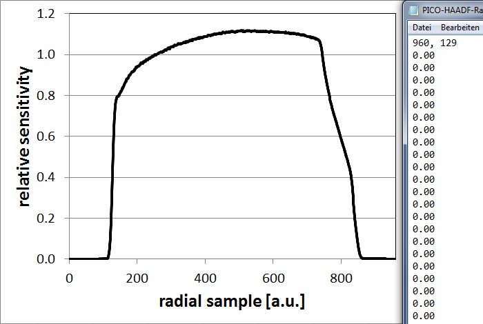
Relative radial detector profile measured for a typical HAADF detector (left) and the first lines of a respective detector sensitivity file.
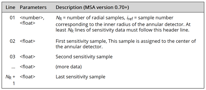
Detector sensitivity files are expected to be text files with a header line consisting of two numbers, and a sequence of lines containing one sensitivity value per line.
The first of two numbers in the header line denote the total number of radial sensitivity samples in the profile (number of lines following, respectively). The second number identifies the reference sample number iref of the profile corresponding to the inner detector radius beta1. In the example shown above, this is sample number 129 of 960. The simulation assumes that the first sample (i=1) corresponds to the center of the annular detector (theta=0) and calculate the sensitivity s at scattering angle theta with the formula
i = 1 + theta · (iref-1) / beta1
s = profile( i )
where i refers to a sample of the provided profile corresponding to theta.
For matching experimental and simulated images on the same absolute intensity scale, re-scaling of both images is required.
1. Determine the average detector response for the same settings controlling the probe current, the detector readout, and the scanning (dwell time) as used for the imaging.
2. Subtract the vacuum intensity level (counts) from the detector image and from the experimental image.
3. Calculate the average response of the detector over the whole active area, and divide the detector response image and the experimental image, both, after subtraction of the vacuum count level.
4. Finally, extract the radial average of the normalized detector image. This should give a curve such as shown above.