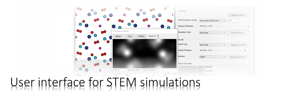
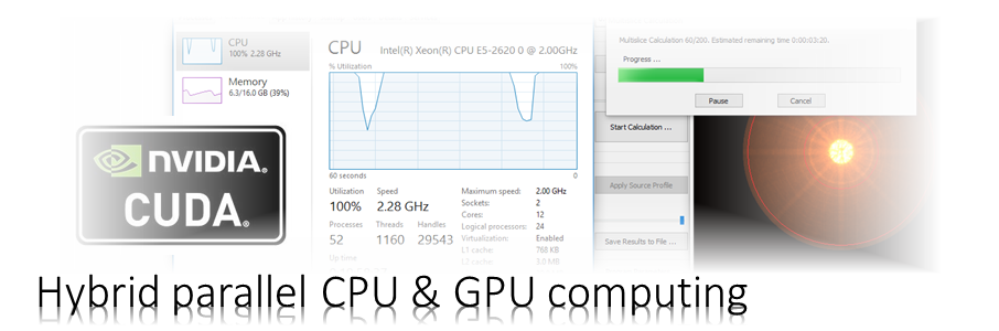
The Dr. Probe graphical user interface (GUI) provides easy access to basic STEM image simulations with direct display of results. Calculations are accelerated by using many CPU threads and your NVIDIA GPU in parallel. The software runs on 64-bit Windows operating systems.
The user interface is build in dialog form with input controls for parameter setup and managing data. Results of simulations are shown in additional data display windows.
Calculations
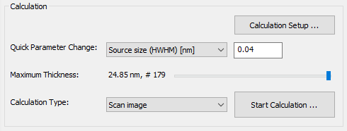
The calculation section of the main dialog provides controls to setup and run multislice simulations.
Most of the calculation parameters are set from the Calculation Setup dialog, which opens when pressing the respective button. There you will find general parameters concerning the calculation, for setting the scan frame, and precession angles.
Important simulation parameters, such as the effective source size, the illumination aperture, the probe defocus, and sample mistilt can be set directly in this section. Select the parameter from the Quick Parameter Change list and edit the values.
The object thickness slider allows you to select the maximum sample thickness between zero and the maximum thickness previously defined in the sample setup. The next multislice calculation will be performed only up to the this selected thickness. By default this slider should be set to its rightmost position. It may be used to quickly reduce the sample thickness for speeding up test simulations.
Before starting a multislice calculation you should select the calculation type from the dropdown list just left to the button labeled [Start Calculation … ]. Three calculation types are supported (version 1.9.2):
Scan image,
Probe propagation & CBED,
and Precession diffraction.
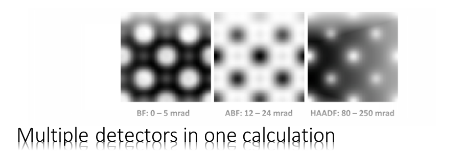
Scan image calculations involve a multitude of multislice calculations for a set of probe positions distributed equidistantly over a rectangular scan frame. Scan images can be calculated simultaneously for a periodic sequence of object thicknesses up to the selected maximum thickness, showing the integrated signal for each detector defined by the detector setup. The calculations are done on a user defined number of CPU cores and on a GPU device in parallel, which may significantly reduce the calculation time if many cores are available.
Calculations of the probe propagation through the sample, CBED pattern, and precession diffraction are done for a fix probe position and with the sampling used for describing the electron wave function. The current probe position is denoted by a white cross in the object data display window and can be changed by mouse click and moving. Alternatively, the probe position can be set explicitly by the scan frame offset in the calculation setup.
Probe intensity distributions are calculated for a periodic sequence of object thicknesses up to the selected maximum thickness. These calculations may include explicitly averaging over thermal atom vibrations (Einstein model), a geometric source distribution, and a defocus distribution in a Monte-Carlo approach.
Calculations are started by pressing the respective button in the lower right corner of the calculation section. A dialog as shown above opens up informing you about the calculation progress and the estimated time until the calculation is finished.

Calculation Setup
The calculation setup dialog as shown in the screen shot below contains 3 tabs allowing input of parameters relevant for
1. multislice calculations in general
2. precession tilt calculations
3. scan image simulations.
Closing the dialog with the [OK] button acknowledges the current input and applies the parameters. Closing with [Cancel] or the [X] in the upper right corner discards any changes made to the parameters.
1. Multislice Setup
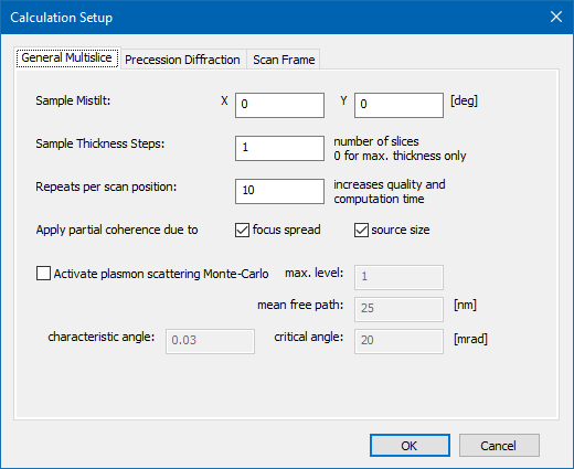
General multislice parameters may apply to all or a sub-set of the available simulation schemes.
Sample mistilt describes small deviations from the zone axis orientation realized by the atomic structure model. The additional tilt is specified here by two parameters in degrees, referring to the X and Y components of sample tilt in the coordinate system of the sample. An approximation is used describing the tilt by tilted free-space propagators [J.H.Chen et al., Acta Cryst. A 53 (1997) 576-589, doi:10.1107/S0108767397005539]. The approximation remains valid for small tilts in the range below 5 degrees.
Sample thickness steps define the step size of periodic detector readout over sample thickness, i.e. along the z axis, in number of structure slices. A step size of 1 would lead to a thickness series where images are extracted with each step of the multislice. With a step size of 2, images would be read out every second slice, etc. When setting the step size to 0 images will only be calculated for the maximum sample thickness of the simulation.
Repeats per scan position specify how often the multislice calculation is repeated at each scan position or for probe propagations and CBED simulations. With each multislice calculated with a different frozen lattice configuration of the sample, the number set here, determines the amount of frozen-lattice averaging. The calculation time will increase with more repetitions.
Switches for focus spread and source size toggle the simulation of partial spatial coherence:
- Scan image simulations, apply the focus spread by explicit averaging if the option is checked here. In this case, each scan pixel needs to be re-calculated with at least the number of focal kernel samples specified in the basic illumination setup. The source size is applied by convolution after the simulation and requires only small additional time.
- Simulations of probe propagation and CBED patterns apply both partial coherence effects by explicit averaging using a Monte-Carlo variation of probe defocus and probe shift. A sufficient number of samples is required especially for representing the 2-dimensional source distribution. The number Monte-Carlo samples is set by the number of Repeats per scan position discussed above. Use 100 or more samples when simulating source size effects.
Activating plasmon scattering Monte-Carlo will introduce additional beam tilts to simulate low-angle scattering in the sample. This strategy effectively implements the approach of B. Mendis [Ultramic. 206 (2019) 112816, doi:10.1016/j.ultramic.2019.112816 ] applying local beam tilts instead of sample tilts. The Monte-Carlo requires 4 input parameters:
– The maximum number of excitations determines how many inelastic scattering events are allowed for each electron while passing through the whole sample. – The mean free path for plasmon excitations in nanometers. – The characteristic angle (mrad) determines the width of the Lorentzian distribution of scattering angles and may be calculated by the fraction Ep/(2 E0), from plasmon energy Ep and primary electron energy E0. – The critical angle (mrad) at which plasmon scattering breaks down. A rough approximation may be Sqrt(Ep/E0).In order to achieve convergence of plasmon Monte-Carlo calculations a large amount of averaging should be used by setting a respectively large number of repeats per scan position.
2. Precession Setup
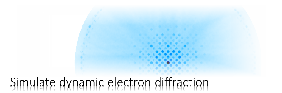
Precession diffraction is a calculation type where a diffraction pattern is integrated while changing the incident beam tilt.
The two parameters define the amount of beam tilt used in a precession tilt simulation where the left value entered refers to the smallest and the right value to the largest tilt magnitude in mrad units.
The precession tilt simulation will calculate how many beams of the numerical diffraction plane fall into the specified range and will calculate a diffraction pattern for each of them with respective incident probe tilt and post specimen de-scan tilt. The resulting precession tilt diffraction pattern is calculated as the total sum of all tilted patterns with a final normalization to the total incident beam current.


3. Scan Setup
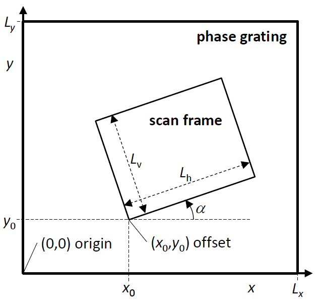
The scan frame parameters define size, sampling, and orientation of the scanning scheme applied in a STEM image simulation. The respective section of the calculation setup dialog provides input fields for the parameters and additional tools automating parts of the setup with reasonable defaults. Dr. Probe uses rectangular scan frames.
The rectangular scan frame is defined by an offset point, by the frame size, and by the frame rotation. The frame parameters are in the coordinate system used to describe the wave function in the multislice calculation. All parameters are denoted in nanometer units with orientations in degrees.
The frame offset is the first scan position and corresponds to the lower left corner of the scan image. Note that orientation of the scan image described here differs from the typical experimental orientation, where the scan image is built up from top to bottom. The scan frame offset can be defined by typing the coordinate into the respective edit boxes. Another way of setting the scan frame offset is by left-clicking in the object data display area, where the scan frame offset is marked by a thick white cross.
The offset position defines also the stationary beam position when calculating images of the probe propagation and CBED simulations. Quick setup tools for scan frame offset and size are provided by three buttons. You can set the scan frame equal to the full slice size, or to half size of the wave function with the option of centering the half frame or keeping its offset at the origin (0,0).
The buttons labeled [Minimum] and [10 pm] provide quick ways of setting the number Nh,v of horizontal and vertical pixels sampling the scan frame. The minimum sampling provides just sufficient resolution based on the current setup of the coherent probe with Nh,v = 4 Lh,v qmax, where qmax = thetamax/lambda, where thetamax is the probe convergence semi angle.
Although no additional information will be generated when scanning with finer steps, a quick way to setup 10 pm scan steps is also provided here. Often experimental images are recorded with around 10 pm scan step on microscopes with 1 Å resolution. The isotropic sampling rate can also be tuned by means of the attached spin control or by specifying its value via the [Set] button.