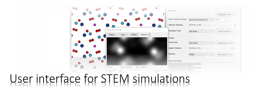
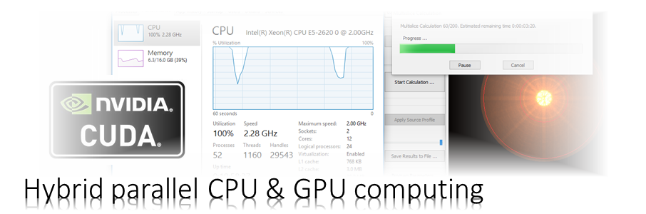
The Dr. Probe graphical user interface (GUI) provides easy access to basic STEM image simulations with direct display of results. Calculations are accelerated by using many CPU threads and your NVIDIA GPU in parallel. The software runs on 64-bit Windows operating systems.
The user interface is build in dialog form with input controls for parameter setup and managing data. Results of simulations are shown in additional data display windows.
Sample
The sample setup is used to input the atomic structure model, create slices of the structure for the multislice calculation and stacking the slices creating a thick sample.
Since object transmission functions can potentially occupy large amounts of working memory, the software keeps no backup of the data. Changes made to the slicing and related data cannot be undone.
The dialog has two tab pages for changing the sample setup. The first page is used to create object transmission functions for slices of an atomic structure model, while the second page is used to stack structure slices generating a thick sample.
Use the [OK] button to return to the main dialog and work with the current sample setup.
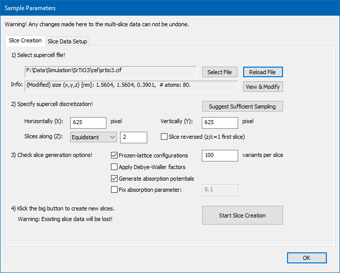
Create Slices
Creating sample data requires a sequence of 4 steps as indicated by the dialog text.
1. Load and modify an atomic structure model
Select a super-cell file containing the atomic structure model describing the sample. Choose either a CEL file or a CIF file for loading.
The selected file will be analyzed and loaded and information about the cell dimension and the number of atoms shown. The structure information from the displayed file name can be loaded again quickly by pressing the [Reload File] button.
It is recommended to always cross-check the loaded structure and in particular the Biso parameters using the Structure modification dialog. Open this dialog by pressing the [View & Modify] button.
Dr. Probe requires an orthogonal super-cell as input for multislice calculations, i.e. a cell were all basis vectors are perpendicular to each other. If your structure has a non-orthogonal unit cell, the software will recognize this and deactivate the further processing of the structure model. Loaded structures can be orthogonalized and re-oriented externally by other programs such as CellMuncher or by pressing the [View & Modify] button.
2. Set the super-cell discretization
The phase grating data to be calculated is sampled in the x–y-plane using a user defined number of pixels. You may choose any number of pixels between 32 and 2048 for the horizontal Nx and the vertical sampling Ny. Higher pixel numbers result in a smaller sampling rate of the projected potentials and enable a calculation of larger scattering vectors. However, the calculation time increases with at least N · Log(N), where N = Nx · Ny is the total number of pixels. In order to keep the calculation time as short as possible you should also take care to use sampling numbers which are products of small prime factors: 2, 3, and 5.
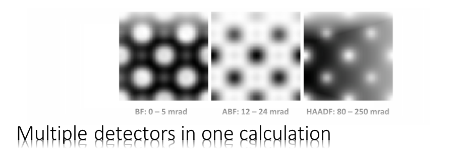
Especially for simulations involving large angle scattering detection, e.g. high-angle annular dark-field STEM (HAADF), the number of pixels sampling the projected potentials may become quite large and need to be calculated in advance. Let s be the size of the super-cell along a certain direction in nanometers, then the sampling rate of the projected potentials is give by the quotient s / Nd, with Nd being the number of pixels used along this direction to sample the potentials. The same sampling rate and size is used later to calculate the propagation of the electron wave function through the object.
The sampling rate defines also the maximum spatial frequency gmax or the maximum diffraction vector qmax with
qmax / lambda ~ gmax = 1/2 · Nd / s,
where lambda is the electron wavelength.
Take into account, that a limiting aperture is applied during the multislice calculation in order to prevent artificial wrap-around of beams in Fourier space producing alias frequencies in the wave function. The aperture blocks all beams with
q > qap = 2/3 · qmax.
The maximum calculated diffraction angle is therefore
qap = 1/3 · N · lambda / s.
Consequently a minimum number of pixels Nmin is required to calculate up to the maximum detection frequency qdet with
Nmin = 3 qdet s / lambda.
The above directives are applied automatically when using the button [Suggest Sufficient Sampling]. This program function automatically sets the number of samples along x and y, taking into account current values of the size of the super-cell, the electron wavelength and the maximum angle of detection. The latter two parameters are taken from the current microscope parameter setup.
The slicing of the orthorhombic structure model along the main propagation direction z of the electron probe can be done in two different ways. A drop-down list lets you choose between a fully automatic scheme, which sets slice terminations at each atomic z coordinate in the structure if not closer to the previous termination than a few picometers. The edit box right next to the dropdown list is deactivated in this case, but displays the estimated number of slices for the current structure. The automatic slicing scheme can potentially create non-equidistant slices. The other option is the traditional equidistant slicing scheme. By choosing this scheme, you can set the number of slices Nz manually. A reasonable number of slices should correspond to the major (001) planes of the atomic structure. The function [Suggest Sufficient Sampling] tries to determine this number automatically from the distribution of atoms along the c-axis of the current super-cell.
The automatic slicing may fail or suggest very large numbers in cases of very complicated structures. It is recommended to check the proposed number of slices carefully. Very large number may lead to serious memory loading and extreme calculation times and are often not reasonable. As a rule of thumb, the average slice thickness (c / Nz) should not be significantly lower than 0.05 nm.
The equidistant sequence of slices begins by default at the fractional coordinate z/c = 0 of the input super-cell and ends with the last slice at the fractional coordinate z/c = 1. You may invert this sequence by checking the option “Slice reversed (z/c = 1 first slice)”.
3. Select options for calculating scattering potentials
Additional options can be selected for the creation of the projected slice potentials. These options control in particular the simulation of thermal diffuse scattering and absorption.
For a frozen phonon calculation you should activate the option “Frozen-lattice configurations” and set the number of frozen lattice variants Nv appropriately. Partial atoms sharing one site by partial occupation will be moved coherently in frozen lattice configurations.
The number of slice variants Nv determines the number of frozen lattice states per slice, which are used to simulate random atomic displacements due to thermal vibrations. The mean atomic vibration amplitudes are calculated from the Debye-Waller parameters B in nm^2 as specified in the super-cell file. For a frozen-lattice calculation, the atomic potentials are displaced by a random distance from the respective equilibrium positions. A good range for the number of frozen-lattice variants Nv per slice is between 10 and 100, depending on the target object thickness, on the scan step size and on the periodicity of the object structure along the projection direction. In principle, Nv should be increased
– for smaller structure periods along the projection direction (smaller number of structure slices),
– for larger object thickness, and
– for smaller scan steps.
By activating the option “Apply Debye-Waller factors” the projected potentials dampened by a Gaussian Debye-Waller factor Exp[- 1/4 B g^2], where g denotes a spatial frequency. This can be a fast alternative for bright-field, low angle electron diffraction simulations with thin samples.
When using Debye-Waller factors, absorptive form factors as proposed by Weickenmeier and Kohl [Acta Cryst. A47 (1991) p. 590-597] are generated when checking the option “Generate absorption potentials“. These potentials provide a fast way to simulate the intensity in the elastic channel for thin and weakly scattering samples.
When not using Debye-Waller factors, absorptive potentials will be generated to account for the electrons scattered to angles beyond the band-width limiting anti-alias aperture of the multislice calculation. The effect of this should be very small for sufficiently large grid sizes in frozen-lattice simulations.
Alternatively you may use the option to apply a “Fix absorption parameter“, which effectively uses a certain fraction of the elastic scattering factor as absorptive form factor, as proposed by Hashimoto, Howie, and Whelan [Proc. R. Soc. London Ser. A, 269 (1962) p. 80-103]. For low-angle scattering calculations and medium Z materials a value around 0.1 is proposed. This is an empirical parameter often used to account for loss of intensity in bright-field and HRTEM simulations.
4. Start the calculation of object functions
Start the calculation process for phase gratings by clicking the button [Start Slice Creation]. Depending on the parameter setup, the calculation will require a significant amount of time and memory. You can approximate the required amount of memory Mslc in bytes by the formula
Mslc = 8 · Nx · Ny · Nz · Nv.
A popup dialog will appear with information on the slice generation progress with an option to abort the calculation. In case of aborting no slice data will be present afterwards, which means that previously existing slice data is lost.
After a successful calculation, new transmission functions are stored in memory and listed in the second page of the dialog for stacking them to a thick sample.
Structure Modification
Layout of the structure modification dialog
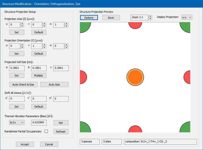
The Structure Modification dialog as shown by the screenshot below can be used to view and modify the structure model currently loaded by the slice creation dialog. The main purposes of this dialog are the orthognalization of non-orthogonal input structures, the re-orientation of the input structure to a specific projection axis and the setup of the physical x–y-frame used by the multislice calculation. The functions provided by this dialog are mainly targeting at the modification of periodic crystal structures without defects. In particular the re-orientation and re-sizing algorithms may not produce reasonable results when the input structure contains defects, interfaces, nano-particles, or amorphous material. Such structures should be modified with other, more specialized crystallography software.
The documentation of the dialog and the implemented functions presented here is done by means of an example structure, which is a cubic SrTiO3 structure as published by Yu.A. Abramov et al. [Acta Crystallographica B51 (1995) 942-951]. The input structure model is provided here by download in form of a CIF file. You can load this CIF file in the slice creation dialog and then open the structure modification dialog by pressing the [View & Modify] button. Doing so, you should receive a similar display of the structure modification dialog as shown in the image above. When opened, a proposal of an orthogonalized version of the input structure is generated for a projection along [001] with minimum size of the super-cell. In the present example, this proposal is identical to the input structure spanning a cubic cell with 3.9 Å lattice constant. The initial display shows the modified structure projection in the x–y-plane. Here, the display options have been setup to show Sr in green, Ti in orange, and O in red color.
The dialog is divided into a left part providing controls and functions to modify structure parameters, and a right part displaying a projection of the modified structure. The modifications are applied to a copy of the structure model currently loaded by the slice creation dialog. When closing the dialog with the [Accept] button the modified copy will replace the previously loaded structure model. Closing with [Cancel] will discard all changes and keep the previous structure model for slice creation.
Structure projection display
The structure display on the right side of the dialog shows a projection of the current modified structure model. A tool tip provides information about the atomic composition below the mouse pointer when moving with the mouse over the display area.
The display window spans the available space in the dialog at 1:1 zoom setting. The zoom setting can be changed in by means of the spin control attached to the edit box denoting the current zoom factor. For zoom factors > 1, the size of the window becomes larger than the available space in the dialog. In this case scroll bars are added to navigate the view port. The structure display always spans over the complete projected super-cell in the chosen projection plane. The two info fields below the image denote the number of atomic species and the number of atomic sites occupied by these species in the modified super-cell.
The projection plane of the structure display can be selected by the drop-down list control in the upper right corner of the display area. Three projections are available. Choosing x–y projects the structure along the c-axis of the modified orthogonal super-cell, which is identical to the chosen projection direction of the image simulation, i.e. the main incident beam direction. The other two projections, x–z and y–z, can be used to determine manually the number of atomic planes along the main incident beam direction, providing a hint on how many slices should be used for the creation of phase gratings from the structure.
The graphical properties of the display, such as background color, colors used for the atomic species, transparency, and borders can be adjusted by an additional options dialog that opens and closes by clicking on the [Options] button in the top-left part of the display area.
The [Save] button provides an interface to store the modified structure model as CIF file or CEL file, or to save the current image in several different graphics file formats, such as JPEG, PNG, or TIF.
Structure modification functions
The orientation of the structure is specified by a ‘Projection Axis‘, defining the new c-axis of the resulting orthorhombic super-cell in terms of an real-space [uvw] vector of the input lattice. The default [uvw] is [001]. You may set an explicit [uvw] vector by clicking the [Set] button below. Spin controls attached to each of the edit controls allow you to change the value by ± 1.
The azimuthal orientation of the structure by rotation around the new projection axis is specified again in terms of a lattice vector [uvw] of the input structure. This ‘Projection Orientation‘ vector defines the new b-axis of the resulting orthorhombic super-cell. Again you may set the components of this vector explicitly or modify it by clicking the attached spin controls. The default vector is [010].
The two vectors, ‘Projection Axis‘ and ‘Projection Orientation‘ fully define the orientation of the new orthorhombic super-cell basis vectors in the system of the input super-cell basis vectors. The definition of the new super-cell is completed by setting its dimension along the 3 new axes. This is done by specifying the a, b, and c lengths of the super-cell in nanometers. With the [Set] button you can enter an arbitrary size of the new super-cell, while the [Multiply] button allows you to grow or shrink the cell along the three axes by certain factors.
The volume defined by the two orientation vectors and by the size of the super-cell will be filled with atomic sites by periodic repetition of the input structure. For this procedure the origin of the new orthorhombic super-cell is identical to the origin of the input super-cell. Whenever one side (axis) of the new super-cell does not coincide with a lattice vector of the input cell, the resulting atomic structure will not be periodic. Since it may sometimes be difficult for beginners to identify commensurable cell sizes, two functions are provided, which try to determine the minimum size of the new super-cell representing again a periodic crystal structure. The function [Auto Orient & Size] determines the smalles possible periodic super-cell for the given ‘Projection Axis‘, with free azimuthal orientation. Pressing the respective button will update the [uvw] components of the ‘Projection Orientation‘ vector as wall as the a, b, and c lengths of the new super-cell. The function [Auto Size] will try to find a the super-cell size for a periodic structure with an azimuth orientation as close as possible to the current [uvw] setting. However, if such a solution is not found for reasonably small super-cell, the [uvw] components may be changed slightly.
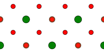
For the present example, we change the ‘Projection Axis‘ to [uvw] = [110] and the ‘Projection Orientation‘ to [uvw] = [001]. After doing so, you will see a strange atomic structure projection with the original cubic input cell size. By pressing the [Auto Size] button, the cell size is updated to an orthorhombic size with a = 0.551685 nm, b = 0.3901 nm, and c = 0.551685 nm. The x-y structure projection image displays now the typical perovskite [110] structure with a row of SrO columns and a row of Ti and O2 columns, as shown by the screenshot.
Structure modification dialog after applying a new orientation of the cubic input structure to a [110] zone axis and updating the new super-cell size with the [Auto Size] function.
Selecting one of the structure projections x–z or y–z shows that the new structure has 4 atomic planes along the z direction, which would require a partitioning into 4 slices for the multislice calculation.
In order to avoid round-off errors in the slicing routine it is sometimes advantageous to shift all atoms along z by one half of a slice, such that the atomic sites of each atomic plane are centred in each equidistant partition of the super-cell along z. In the present case with 4 atomic planes and therefore preferably also 4 slices the amount of shift to be applied along z would 0.125. A shift of the atomic structure in fractions of the new super-cell lattice can be set by the components of a [u’v’w’] shift vector below the ‘Auto Size‘ functions on the left side of the dialog. The shift-vector can only be set explicitly and denotes the amount of shift in fractions of the new super-cell size. Thus, if the cell size is changed, the same fractional shift corresponds to a different absolute shift vector. Take care to update a non-zero shift vector manually whenever you change the super-cell size. The default shift vector is [000].
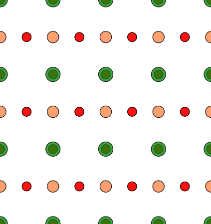
For the present example we also extend the new super-cell by a factor of 2 × 3 × 1 along its three axis using the [Multiply] button. Since the cell size along the new c axis is not modified by this extension, we do not need to update the shift vector [u’v’w’] = (0, 0, 0.125). The x–y and the x–z projection of the final super-cell is displayed in the image.
SrTiO3 extended by 2 × 3 along x and y in x–y projection (top) and x–z projection (bottom). Due to the shift of the atomic structure by 1/8th along the c axis of the super-cell, the atomic planes are centered in each of the 4 equidistant partitions along z.
Below the controls for the shift vector setup, you find controls to manage the thermal vibration parameters of each atomic species in the structure model. The dropdown list control on the left contains all atomic species of the modified structure. The info box to the right of the dropdown control displays the Biso parameter of the selected atomic species in Å2 units. You may change the selected Biso parameter by clicking the [Set] button right of the info box.
By activating the ‘Randomize Partial Occupancies’ switch, the partial occupation of atomic sites contained in the modified structure will be changed to a full occupation variant. Already fully occupied sites will not be affected. Sites with a partial occupation against a partial vacancy will be changed randomly into a fully occupied site or a vacancy site. Sites occupied partially by multiple atomic species will be changed into a site fully occupied by a single species. The selection of occupation is done by means of random choice, which orients on the occupation levels defined by the input structure model. Another random occupation variant can be created by pressing the [Refresh] button to the right of the check box.
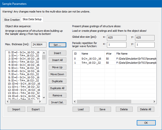
Stack Sample Data
Stacking pre-calculated object transmission functions (slices) determines the maximum sample thickness of the simulation.
Setup a sequence of slices as it should be used during the multislice calculation from the entrance plane to the exit plane. The stack will be shown in the list on the left side, while slices available for stacking are listed on the right side.
In its upper part, the dialog denotes the sampling of the available slice data.
There are two edit boxes to set a periodic repeat along the x– and y-axis. This repetition can be used to increase the number of pixels of the calculated wave function beyond the present sampling of the projected potentials, e.g. to increase the number of pixels sampling the bright-field disk in CBED simulations. Use this option with utmost care, i.e. use only small numbers.
Available slice phase gratings listed on the right are identified by ID numbers as shown in the first column of the list. Further, a slice name, the number of frozen-lattice variants, and a file name may be displayed. The slice name denotes the composition of the slice.
The object slice sequence on the left side is a sequence of phase grating IDs and determines the sequence of the slices applied in the multislice calculation. Use the set of buttons between the lists to manipulate and build the sequence.
The length of the object slice sequence determines the maximum sample thickness of the calculation, which is denoted in the info box above the list. A longer list will not cause increased memory consumption but will result in longer calculation times.
The easiest way of setting up a thick sample is to use the [Set …] button next to the Max. thickness display. You can set the desired sample thickness in nanometers and the program will fill the slice list on the left side with a periodic sequence of the slices on the right side.
Controls for individual slice stacking (left list)
[Insert]
The slices selected on the right side are inserted above the selected position on the left side. In order to insert selected slice at the end of the current sequence, undo any selection in the left list. You can toggle selections individually by mouse clicking the respective item while holding the Ctrl (Strg) key.
[Insert All]
All slices on the right side are inserted above the selected position on the left side. The slices are appended to the end of the object slice sequence if no selection is made in the left list.
[Move Up]
Slices selected on the left side are moved up by one position in the sequence towards the entrance plane.
[Move Down]
Slices selected on the left side are moved down by one position in the sequence towards the exit plane.
[Duplicate]
The slices selected on the left side are duplicated and inserted above the currently selected position into the slice sequence.
[Duplicate All]
All slices of the object slice sequence are duplicated. The complete object structure is thus repeated along the projection direction.
[Remove]
The slices selected on the left side are removed.
[Invert Sel.]
The selected slice sequence is reversed in its top-down order.
[Import]
Loads an object slice sequence from a text file.
[Export]
Saves the current object slice sequence to a text file. You may reload the sequence again later by using the [Import] function. You can also insert the content of the file at the respective position of a parameter file for the command-line program MSA.
Controls handling slice data (right list)
Slice data as listed on the right side can be loaded from disk files, saved to files, removed from the list, and merged to one slice. For each of these functions a respective button is present below the list. The list manipulation supports multiple selection.
[Load]
Slice files saved previously can be loaded and used again. You should check that the slice data corresponds to the current program parameters, especially to the current accelerating voltage. Take care to load only slice data, where all the slice have the same sampling and corresponding physical dimension. The slice-to-slice consistency in terms of sampling parameters is not checked by Dr. Probe.
[Save]
By saving slice data to files you may use them again later or by the command-line tool MSA.
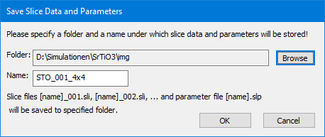
Select the desired destination folder and specify a unique file name. Existing files with equal file names will be replaced by the new files without asking your permission. Clicking the [OK] button to start the saving and wait until it is finished.
One file is saved for each slice with a file name is composed of the user specified name followed by a separator character (_), and a three-digit number identifying the position of the slice data in the list. One slice file may contain many slice variants as used for a frozen-lattice calculation. An additional collection of slice parameters is saved next to the slice files in form of a text file with extension ‘.slp’.
[Delete]
The slice data selected in the available slice data list will be unloaded from the working memory and the respective items will be removed from the list. Any slice inserted to the object slice sequence on the left side having the same ID as the removed item, will be removed automatically.
[Delete All]
All slice data will be unloaded and both lists, the object slice sequence and the available slice data will be empty afterwards.