The program MSA calculates the diffraction of fast electrons in an atomic structure with the multislice algorithm. The results can be complex-valued wave functions, STEM images, CBED patterns, or probe intensity distributions.

MSA
The program is compiled for single-thread calculations and can be called from command-line shell or from other programs on 64-bit operating systems (Microsoft Windows, Linux and Max OSX). It is controlled via a parameter list provided in a text file and by calling options.
Examples
STEM image simulation controlled via parameter file:msa -prm msa.prm -out STEMimage.dat
STEM image convolution with a specific geometric source size:msa -prm msa.prm -in STEMimage.dat -out STEMimage_convoluted.dat -sr 0.06
4D-STEM simulation controlled via parameter file storing a thickness series of CBED patterns for each scan pixel:msa -prm msa.prm -out 4D-STEM.dat /3dout /pdif
TEM exit-plane wave function:msa -prm msa-tem.prm -out wavefunc.dat /ctem
TEM exit-plane wave function with object tilt:msa -prm msa-tem.prm -out wavefunc_tilted.dat -otx 5.4 -oty 1.5 /ctem
Multislice
The multislice algorithm is used for calculating the electron diffraction by the electrostatic potential of an atomic structure [J.M. Cowley and A.F. Moodie, Acta Cryst. 10 (1957) p. 609-618]. In this approach the scattering by a thicker sample is described as a sequence of scattering events on thin sample slices taken along the main direction of the incident electrons. Between the scattering events, the electron wave function is propagated in free space towards the next slice.
The approach of sequential scattering and propagation can be implemented in an efficient numerical form. The the scattering of electrons from projected slice potentials is a multiplication of the electron wave function with an object transmission function (phase grating). The subsequent free-space propagation to the next slice plane is calculated by a multiplication of the scattering result with a propagator function in Fourier-space. The calculation for a thick sample comprises thus two multiplications, one forward and one inverse Fourier transform for each structure slice.
MSA supports frozen-phonon calculations as well as calculations with absorptive potentials. Frozen-phonon configurations of the scattering potentials are expected to be pre-calculated e.g. by the program CELSLC or the Dr. Probe GUI and are stored in input slice files. During the calculation MSA selects and applies a random frozen-phonon variant of each slice. By this way, each single multislice calculation, e.g. for each STEM image pixel, is effectively calculated with an individual frozen-phonon configuration of the whole sample (detailed description: see below).
STEM or coherent TEM
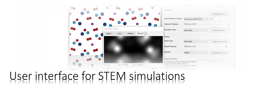
Calculations for STEM and TEM differ by the form of the incident wave function and by the way how the electron wave function obtained at the exit-plane of the sample is transferred into image intensities.
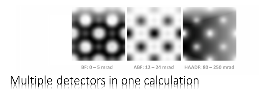
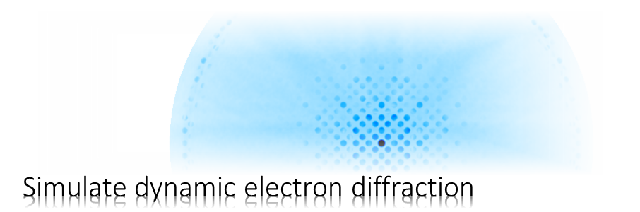
For STEM image calculations, the incident electron wave function is converging into a focused probe and scanned over the sample. For each probe position, the wave function below the sample is analyzed in diffraction space, where the absolute square is integrated for given detector areas, generating STEM images. This means that MSA can be used in its default STEM mode to calculate STEM images, CBED and even scanned CBED (aka. 4D-STEM) data sets.
For TEM image calculations (option /ctem), the incident electron wave is approximated by a plane wave and the electron wave below the sample is passed further through imaging optics towards a detector where the absolute square is taken in real space. In the TEM case, MSA can be used to calculate the electron wave function below the sample (exit-plane wave function). The calculation of TEM image intensities including the application of wave aberrations, partial coherence and incoherent contrast dampening effects are done by the program WAVIMG, which is also available with the Dr. Probe software package.
Frozen-lattice variation procedure
Thermal atom vibrations have a significant effect in electron diffraction since they represent a deviation of the atomic object structure from the ideal symmetry of a crystal. When aiming for a quantitative evaluation of electron diffraction experiments by comparisons to simulations, the simulations have to consider the effects caused by thermal lattice distortions, which are frequently addressed as thermal diffuse scattering (TDS). The main difficulty for the incorporation of the related effects is that the approximations made to speed up electron diffraction calculations, be it by means of Bloch-waves, or by the multislice algorithm, assume an object with fix atom positions.
One can distinguish between two main routes for the consideration of TDS for the calculation of the elastic electron diffraction:
1. Modification of the object scattering potential by Debye-Waller factors (DWF), and
2. Averaging over repeated calculations using different frozen states of the crystal lattice (frozen lattice / frozen phonon).
The first route is a quasi-coherent approach, where, the atomic scattering factors are convoluted by a Gaussian function approximating the distribution of atomic displacements. The elastic electron diffraction is then calculated using the modified potentials, effectively reducing the structure factors due to the deviations from the ideal crystal structure symmetry. This approximation disregards any type of incoherent and diffuse scattering power. The respective loss in the inelastic scattering channel is usually registered by an absorptive form factor. For thin samples is also possible to include the contribution of TDS in such a calculation [3].
The main drawback of the application of DWFs is that the large angle scattering, as recorded by a high-angle annular dark-field (HAADF) detector, is massively compromised. Nevertheless, the application of DWFs is the most efficient approach for the calculation of bright field electron diffraction and is very frequently used for the calculation of coherent TEM images.
The second route provides a more realistic simulation of the electron diffraction also to larger scattering angles. The frozen lattice approximation is based on the assumption that each electron interacts with a specific static scattering potential. This assumption is in so far justified, since the velocity of the incident electrons, which is usually around one half of the speed of light for medium voltage electron microscopes (100 – 300 kV), is by several orders of magnitude larger than the speed of atoms due to thermal vibrations. In this view, each electron is scattered by a different frozen state of the lattice. The detected signal, to which up to several thousands of scattered electrons contribute, registers thus information from a large amount of different frozen lattice sates. Depending on the available data on the thermal vibration of the investigated crystal, an explicit phonon dispersion can be considered (frozen phonon approximation). Without specific information about the excitation of vibrational modes, usually incoherent atom vibrations are assumed (frozen lattice approximation). In both scenarios, usually a repeated computation of the electron diffraction is required, which amounts to a significant computation time when the system size is large, such as for large angle scattering calculations.
A time-efficient implementation of the multislice algorithm is applied by Dr. Probe. The implementation allows the simulation of thermal diffuse scattering using the frozen lattice approach. A set of M frozen lattice states is pre-calculated for each of the N object structure slices. The object slices are chosen as thin as possible containing preferably only one atomic plane. Projected potentials are calculated for all frozen states including random atom displacements to represent thermal atom vibrations. During one run of the multislice calculation one of the M pre-calculated frozen states of the current slice is selected randomly from the respective set of M states and applied to the current wave function in form of a phase grating. A random permutation of the pre-calculated frozen states is produced by repeated application of this random selection scheme over the whole sample thickness as illustrated by the figure below.
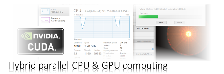
By this way one obtains free control over the number of frozen states applied to a scan pixel during run-time without additional calculation effort. The procedure allows for example to adapt the number of averaged frozen states locally depending on the local signal variation and thereby to optimize the total calculation time in conjunction with an improved simulation precision. A fast run-time variation of frozen states requires a previous loading of all pre-calculated frozen states (phase-grating slices) into the computer working memory. However, a large number of phase-grating pixels and frozen lattice states can be handled with commercially available computers supporting more than 4 Gigabytes working memory.

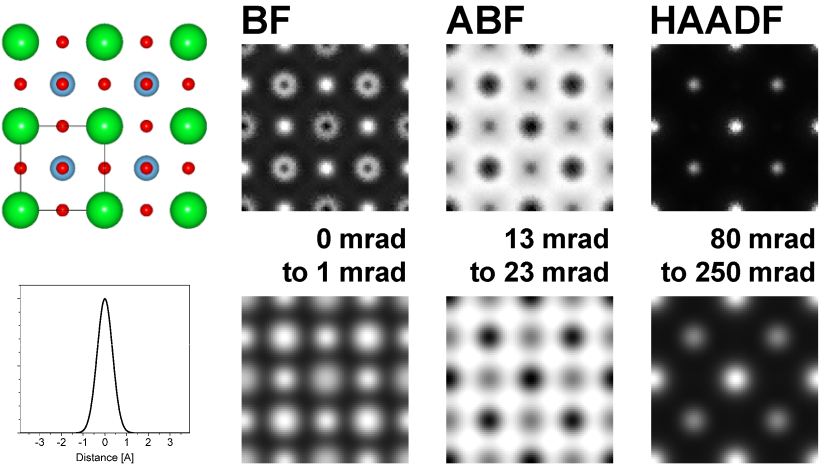
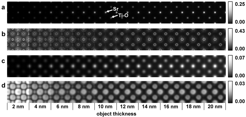
A minimum calculation time for a scan image is obtained by using only one random permutation of frozen slice states per scan pixel. As expected, this approach leads to a strong variation of the detected intensity per scan pixel. The intensity variation from pixel to pixel is visible in the upper row of the below figure, showing images composed of 40 x 40 scan pixels per projected SrTiO3 [100] unit cell. For this simulation example, only one frozen lattice permutation of the object consisting of 25 unit cell periods (50 slices) was contributing to each pixel. However, the individual scan image pixels where calculated with different combinations of frozen lattice states made up from M = 50 pre-calculated frozen states for each of the two super cell slices.
A subsequent convolution of the images with an effective source profile is required to obtain qualitatively and quantitatively correct images [4]. The images of the lower row in the figure below are obtained by convolution of the respective upper row images by a Gaussian source profile of 0.5 A 1/e-half-width. The convoluted images appear smooth and represent also an average over frozen states applied to neighbor pixels within the effective source radius (convolution radius).
This a-posteriori averaging of frozen states is possible due to a sufficiently small simulation scan step. In the present example, the scan step is approximately 10 pm per pixel, which is close to experimental scan steps frequently applied in high-resolution STEM. A sufficiently small scan step for a-posteriori frozen state averaging depends on the number of pixels per intensity peak in HAADF images before convolution and on the number of pixels within the effective source area for BF and ABF images.
Results of statistical evaluations from 90 independent calculations show a significant decrease of the pixel intensity variation after source profile convolution from approximately 40% down to 3% of the pixel mean value (see figure above). This precision level is sufficiently small for a comparison of simulation and experiment especially, when analyzing integrated column intensities. In conclusion, the consideration of just one frozen state per pixel is sufficient to obtain quantitatively meaningful simulation data when using realistic scan steps and subsequent source profile convolution.
References
[1] J.M. Cowley and A.F. Moodie, Acta. Cryst. 10 (1957) p. 609.
[2] R.F. Loane, P. Xu, and J. Silcox, Acta Cryst. A 47 (1991) p. 267.
[3] A. Rosenauer, M. Schowalter, J.T. Titantah, D. Lamoen, Ultramicroscopy 108 (2008) p. 1504.
[4] C. Dwyer, R. Erni, and J. Etheridge, Ultramicroscopy 110 (2010) p. 952.