This part of the PantaRhei documentation describes how the program is used by means of an example. The example documentation is divided into the following section:
- Starting the software
- Importing stability measurements from log files
- Extracting the characteristic function
- Model-based lifetime evaluation
- Export of images and data
You may follow this example on your computer. All necessary input data is provided by download (see red button above).
1. Starting the software
Start PantaRhei by clicking on the respective link in your Windows startup menu, or by double clicking the executable binary PantaRhei.exe from an explorer window of the installation folder. If you have installed PantaRhei with the installer script you may alternatively type “PantaRhei” int the run edit box of the Windows startup menu.
PantaRhei should show up with its main dialog window as shown by the screenshot below. An additional splash screen appears. You may close the splash screen after two seconds with a mouse click, or it will close automatically after a few more seconds.
The main dialog of the user interface is organized in essentially four section along the vertical direction:
1. A menu bar provides access to all available program functions.
2. The time-astigmatism series section provides controlls to load, select, and manage multiple measurements
3. The major area contains a tabbed data view to display input and output data in text and graphical form.
4. The message log displays program processing information, warnings, and errors.
Right after the start, PantaRhei checks its registration status. In case of a valid registration, the registration information will be displayed in the message log as shown by the screenshot above. If no valid registration information is found, a registration dialog will always pop up during the program launch asking to complete the registration. A detailed instructions on the registration procedure are given in the download section of this website. The registration information will be stored in the global application data folder of your Windows OS, i.e. in the folder “C:\ProgramData\PantaRhei\”. The registration concerns the installation of the program on a specific computer and is valid for all users of this computer.


2. Importing stability measurements
The stability evaluation begins with importing an existing measurement log file. For your convenience an example log file is provided here for download. The data of the example log file has been recorded with a FEI Titan 80-300 TEM operated at 300 kV accelerating voltage. In this operation mode, the microscope has an information limit of better than 1 A. The astigmatism data was extracted from 1075 images of an amorphous Tantalum film using the ATLAS software. The image seried was recorded over more than 12 minutes without any operator action and contains 1075 images.
The log file is imported by clicking on the [Import] button in the main window, by selecting the Import Data Log… iten in the File menu, or by pressing the Ctrl+L key combination.
A file-open dialog pops up as shown above. Select the type of log file using the provided dropdown list. This selection has to be made to specify the specific format in which data is stored in the log file. Selecting the wrong log format will cause the import procedure to fail. The example provided in this documentaion is a log file created with the ATLASstab tool. Then browse to the location of the log file on your hard disk and select the log file. Finally, click the [Open] button (label adopts to the language of your operating system), which will initiale the log file import.
When the log file has been successfully loaded and the log data has been interpreted, the measurement is added to the list of time astigmatism series. The data series list provides general information such as number of images, total recording time, and recording frequency in order to distinguish between multiple loaded measurement data. If more than one measurement has been loaded, you can switch between the measurements, by selecting the active measurement from the drop-down list. Individual series can be unloaded by pressing the [Delete] button. Unloading of all series at once is done by pressing the [Delete All] button in the main window.
Just after loading a measurement two tabs appear in the central area of the main window as shown by the screenshot below. When selected, the leftmost tab “Log Text” displays the content of the imported log file in text form. The second tab “A22-Time Graph“, which is selected by default after the import, shows a diagram of the astigmatism components A22-x (red) and A22-y (blue) over time. An identical scale is chosen for the two astigmatism components.
Alternatively the imported astigmatism data can be displayed in a 2-D astigmatism plot, omitting the time dimension. The plot display type is selected using the dropdown-list on the right side of the diagram area.
Basic series statistics are displayed, such as the average, standard deviation and mutual correlation of the two astigmatism components. The second line of the series statistics reports the angle of rotation of the 2-dimensional astigmatism plane, where the astigmatism x- and y-components would appear uncorrelated. You can rotate the astigmatism plane by setting a rotation angle in the edit box on the right side of the diagram and by pressing the [Re-Extract] button. You may also mirror the y-component by checking the respective box and pressing the [Re-Extract] button again.
Proceeding with the evaluation of the astigmatism evolution with time requires a valid registration from this point on. Nearly all functions described below are disabled for an unregistered copy.
3. The characteristic function
The first step of the evaluation procedure is the extraction of a characteristic function from the imported time-astigmatism series. The extraction is started by pressing the [Char. Function…] button in the “A22-Time Graph” tab, by clicking the Evaluate Characteristic Function item in the Analyze menu, or by pressing the Ctrl+F key combination.
The characteristic function is calculated by means of three data transformations and a final substraction of an extrapolated measurement error. The first data transformation is made by extracting astigmatism differences between pairs of data points. Due to the continuous acquisition, each pair of data points corresponds to a certain timespan. As the second data transformation, the respective astigmatism difference for a pair of data points is squared. The third transformation is done by averaging over all squared astigmatism differences belonging to the same timespan. In this transformation scheme, short timespans are represented by much more statistically independent data pairs than long timespans. The minimum number of data pairs (diversity) required for the extraction of the characteristic function can be set in the Program Parameters, which are accessible via the Settings menu. Keep in mind, that a higher minimum diversity will reduce the maximum timespan of the characteristic function, but will improve the statistical significance of the curve. A smaller minimum diversity will reduce the statistical significance but extends the extraction towards longer timespans. An extrapolation based on a reduced statistical significance can be highly speculative.
The characteristic function is finally obtained by substracting an average statistical error estimate of the astigmatism measurement. The estimate of the statistical measurement error is obtained by extrapolating the uncorrected data linearly towards the timespan t = 0, where hypothetical differences between two data points should be just because of measurement errors. On the quadratic scale, the average difference of the apparent astigmatism for a given timespan is a sum of the actual average squared astigmatism change and the average squared measurement error. The latter can thus be eliminated from the average data curve.
The characteristic function of the present example, as shown in the screenshot above, has been extracted with a minimum diversity of 15. After extraction, the “Charact. Func. tab is enabled and selected automatically. A convenient set of points of the characteristic function is plotted as black dots in a diagram with the timespan on the abscissa and the squared astigmatism difference on the ordinate.
The two fields above the diagram denote general properties of the extracted characteristic function, such as the number of data points, the maximum timespan, and the extrapolated and removed statistical error (1-sigma r.m.s) of the astigmatism measurement.
A statement on the lifetime of the optical state is made directly from the characteristic curve. The lifetime is identified as the timespan, where the characteristic functions exceeds tolarable astigmatism change. The astigmatism tolerance is given in nanometers and has been determined from the electron energy, the target resolution, and an astigmatism phase-shift tolarance. While the first two parameters can be set on the right side of the diagram area, the phase-shift tolarance is specified in the program settings. After changing one of the parameters, you can repeat the direct lifetime estimation with updated parameters by pressing the [Refresh] button.
The direct lifetime estimation is limited to the maximum timespan of the characteristic function. In the present example, the image series does not provide a sufficient amount of data to determine the characteristic function beyond a timespan of approximately 50 s. For timespans below 50 s, the characteristic function doesn’t exceed the tolerated astigmatism change for 300 keV electrons, 0.8 A target resolution, and Pi/4 phase-shift tolarance. Given these parameters, one can just state that the lifetime of the optical state is likely to be larger than 50 s.
A “Summary” tab is generated, which presents the major results of the stability evaluation in text form.


4. Model-based lifetime evaluation
The limitation of the direct evaluation method to the maximum timespan of the charcteristic function is overcome by a model-based approach. The model-based evaluation method allows you to extrapolate the characteristic curve towards longer timespans.
Two contributions leading to a variation of the twofold astigmatism over time are considered by the applied model: (i) a random-walk and (ii) a constant drift. Using the model-based lifetime evaluation, the two contributions can be separated. Due to the random-walk component, the astigmatism variations have a large variance, which results in quite large error bars compared to the average, which is characteristic function. A very useful output of the model-based evaluation is a probability curve, which informs you about the chance to still work in a once adjusted state after a certain timespan.
Start the fully automated model-based evaluation by pressing the [Fit Model] button in the “Charact. Func.” tab, by selecting the item Fit Model in the Analyze menu, or by pressing the Ctrl+M key combination.
The upper image on the left shows a screenshot of the Fitted Model display, where the timespan abcissa is now extended such that the extrapolation of the fitted model violates the astigmatism tolerance. The “Fitted Model” tab is automatically selected after the fit. Black circles represent a selection of points of the characteristic function. The thicker blue curve shows the fitted model, while the thinner blue curves represent the 68% confidence band of the data variation around the characteristic function. The horizontal black line denotes the currently considered astigmatism variation tolerance on the squared scale of the ordinate, while the vertical black line marks the timespan, where the fitted model curve violates the astigmatism tolerance. This timespan is extracted as the lifetime of the optical state.
The two boxes above the diagram denote the list of model parameters, the lifetime estimated from the fitted model, and the considered astigmatism tolerance. The latter value can be changed as described in section 3 by setting a different electron energy or target resolution and pressing the [Refresh] button.
In addition, a second plot is generated showing the decaying probability to still work in a once adjusted state after a certain timespan. The probability plot is displayed by selecting the “Prob. Plot” tab in the display area. The probability plot as shown by the second screenshot on the left displays the probability curve in blue. The horizontal and vertical lines denote the timespan, where the probability has decayed to 50% (median), i.e. they mark the timespan after which it is perfectly undecided if the optical state has survived or not.
Also the result summary is updated providing now also detailed information about the fitted model and the best fitting model parameters. The test content of the “Summary” tab can be selected and copied.
5. Exporting images and data
The diagrams and the underlying data can be exported to files by either using the respective Export … items of the File menu, or by clicking with the right mouse button in the image area.
Images of the diagrams can be saved in four common graphics file format: JPG, PNG, TIF, and BMP.
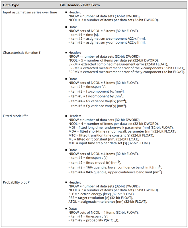
By exporting a data table, the data drawn in the current diagram is witten to a text file in human readable table form. Such tables can be imported by other programs, such as Excel or Origin.
By exporting binary data, the data drawn in the current diagram is witten to a file in raw binary form. Depending on the exported data, the file contains a specific header and data form. A short summary of the generated binary data is listed in the table on the right.