
|
HRTEM image simulation of [110] SrTiO3 |
|
This online example demonstrates the simulation of coherent TEM images of a cubic perovskite SrTiO3 crystal in [110] orientation using the Dr. Probe command-line tools.
The main purpose of this example is to show the basic concepts and functions of TEM image simulations with Dr. Probe step by step, such that it may serve as a template for your own work. The applied simulation approach is kept to a minimum of computational effort, while reproducing realistically the dynamics of elastic electron diffraction and partially coherent imaging by a modern aberration-corrected TEM.
It is however required, that you have installed the Dr. Probe software package properly following the installation instructions available on this website.
TEM image simulations with Dr. Probe are composed of three major steps
which separate the creation of important intermediate data. This separation
allows a few short-cuts when doing parameter variations, as not all
steps need to be repeated depending on the level where the parameter
variation takes place.
Each of the three step is performed by calling a particular command-line tool:
- CELSLC - creating phase gratings of object slices,
- MSA - multislice algorithm calculating the electron diffraction
- WAVIMG - image calculated from an exit-plane wavefunction
For reproducing the individual steps below, it is recommended that you create an empty folder on your hard drive where all intermediate data will be stored, e.g. 'C:\Simulations\Example03'. This folder is used as the working directory for all the example steps, especially for the calls of the three command-line tools.
Simulation targets
Before starting with a simulation it is important to denote the aims
of the simulations and to clarify the involved parameters concerning
the material and the microscope.
For the present example we want to calculate high-resolution TEM
images of cubic perovskite SrTiO3 in [110] zone-axis
orientation considering a spherical-aberration corrected 300 kV
transmission electron microscope with 0.8 Angstrom resolution.
The example will demonstrate the calculation of a single image, the
calculation of a through focus image series, and the computation
of a focus-over-thickness map. The images will be saved to files on
the hard disk containing image intensities as raw binary data.
Object structure data
The object structure for the following TEM image calculations is identical to the structure data created by an example procedure documented on this website. You may follow this example and create the structure definition (CEL) file from scratch, or you can download the structure files here and use it blindly. The structure data is a super-cell of SrTiO3 in [110] zone-axis orientation, which contains a volume of 2 unit cells as displayed in the image below.
 structure model parameters
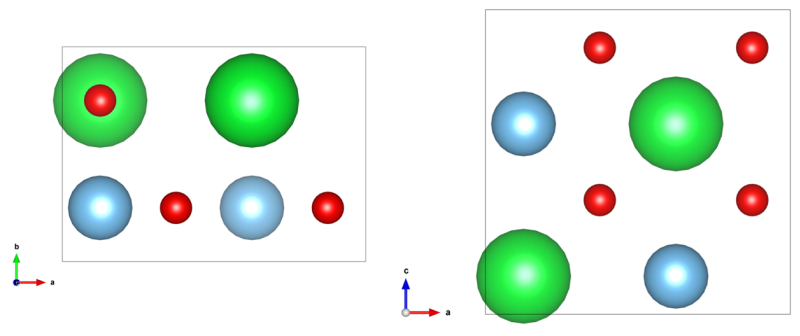
[Left: x-y-projection and right: x-z-projection of the input structure]
Alternatively, you may copy the following text defining exactly the same structure and store it as a structure definition file (CEL) named 'STO_110.cel' from your text editor.
# SrTiO3 [110] super-cell data created by BuildPrimitiveCell and CellMuncher
0 0.5523 0.3905 0.5523 90.0000 90.0000 90.0000
Ti 0.124955 0.250000 0.624910 1.000000 0.005100 0.100000 0.100000 0.100000
Sr 0.124955 0.750000 0.124955 1.000000 0.006600 0.100000 0.100000 0.100000
O 0.124955 0.750000 0.624910 1.000000 0.010800 0.100000 0.100000 0.100000
O 0.374933 0.250000 0.374933 1.000000 0.010800 0.100000 0.100000 0.100000
O 0.374933 0.250000 0.874978 1.000000 0.010800 0.100000 0.100000 0.100000
Ti 0.624910 0.250000 0.124955 1.000000 0.005100 0.100000 0.100000 0.100000
O 0.624910 0.750000 0.124955 1.000000 0.010800 0.100000 0.100000 0.100000
Sr 0.624910 0.750000 0.624910 1.000000 0.006600 0.100000 0.100000 0.100000
O 0.874978 0.250000 0.374933 1.000000 0.010800 0.100000 0.100000 0.100000
O 0.874978 0.250000 0.874978 1.000000 0.010800 0.100000 0.100000 0.100000
*
Please, make sure that the structure file 'STO_110.cel' is now located in a sub-folder named 'cel' of the working directory.
Using CELSLC to create phase gratings of the periodic object structure
The first step of a simulation is the preparation of object transmission
functions, so-called phase gratings, with the program CELSLC providing
the input for the subsequent calculation of the electron diffraction
with the program MSA.
In this step, the object structure model is
partitioned into a set of equidistant thin slices along the later
projection direction, which is always along the c-axis of
the structure model. The slices are ideally thin enough, such that each
contains only one atomic plane. Slicing the object coherently with the
atomic planes ensures that higher-order Laue zones are reproduced correctly
by the multislice calculation. Potentials describing the elastic scattering
of electrons from each slice are then calculated for a given electron energy
and projected along the c-axis to the lower plane of the respective slice.
The projected potentials are finally transformed into an object transmission
function with approximations for weak potentials and forward-scattering,
taking into account an interaction constant.
The program CELSLC samples the object transmission functions on an orthogonal grid of points and includes a relativistic correction of the electron scattering depending on the primary electron energy. Please note that the program expects an orthogonal super-cell as input. If your input structure is not at least orthorhombic, make sure to transform it to an orthorhombic super-cell using for example CellMuncher. You may follow the example procedure on this website describing the orthogonalization of a structure model of AlN. Together with the object structure model, the number of samples, the number of slices, and the electron energy (microscope high-tension) are required input parameters of the program. A full description of all program parameters can be found in the online documentation of CELSLC.
The output of CELSLC is a series of so-called slice files (*.sli), which
constitute the first intermediate data of our simulation example and
will be saved to disk.
As I typically organize the different intermediate data in separate
sub-folders of the working directory, please follow me here by creating
a subfolder 'slc' in your working directory for this example using the
command
md slc
or use the system file explorer to create this folder.
Start the slice creation by calling CELSLC in the following way from the command-line shell:
celslc -cel cel\STO_110.cel -slc slc\STO_110_300 -nx 128 -ny 90 -nz 4 -ht 300. -abs -dwf
The program will inform you about the read input data. In the present
example, it denotes sampling rates of (0.00431484, 0.00433889, 0.13807499)
nm per pixel / slice along the three dimensions of the super-cell. Four
files 'STO_110_300_*.sli' containing object transmission functions will be
stored in the sub-folder 'slc' as specified by the option
-slc slc\STO_110_300.
A fine sampling of the object transmission functions is chosen here with the options
-nx 128 -ny 90. In order to obtain a fast computation, you
should choose numbers with prime factors 2, 3, and 5. The sampling numbers
should be large enough to calculate all relevant diffracted beams. Usually
sampling rates around 0.005 nm/pixel are sufficient for this purpose.
The number of slices was chosen here with the option -nz 4
equal to the number of atomic planes in the super-cell as visible in the
x-z-projection of the structure images above.
With -ht 300. the high-tension parameter specifies an electron
energy of 300 keV to be used for the calculation of elastic electron
scattering potentials. With the option -dwf the atomic form
factors are convoluted by Debye-Waller factors, and the option
-abs triggers the calculation of absorptive form factors
according to Weickenmeier and Kohl [Acta Cryst. A 47 (1991)
p. 590-597]. The absorptive form factors account for the loss of electrons
in the elastic channel due to thermal diffuse scattering.
Calculating exit-plane wavefunctions with MSA
The second step of a TEM image simulation is the calculation of electron diffraction. We apply here a multislice algorithm as proposed by Cowley and Moodie [Acta. Cryst. 10 (1957) p. 609]. This algorithm is implemented in the program MSA of the Dr. Probe package. Please take a look at the online documentation of MSA an study the list of required and optional program parameters.
As required parameters MSA expects that you specify the name of a parameter
file and the name of an output file. All calculation parameters are set up in
the parameter file. The only other program parameter used here is the
option /ctem, which tells MSA to start with a plane incident
wavefunction for conventional TEM image simulation, rather than with a
convergent electron probe as used in STEM image simulations.
The major work in this step is to create and write the parameter file for MSA. As the program can be used for TEM and STEM simulations, only some of the lines in this file are actually used in the present example.
Let's now create such a parameter file in a new subfolder named 'prm' using the command
md prm
or by using the system file explorer! Then store the text block below in a file named 'msa.prm' or download the MSA parameter file and store it in the sub-folder 'prm'.
'[Microscope Parameters]'
1.0 ! [mrad] illumination cone half-angle ! STEM only
0.0 ! [mrad] inner detection angle ! STEM only
20.0 ! [mrad] outer detection angle ! STEM only
0, 'prm\detectors.prm' ! flag and name of STEM detector file ! STEM only
0.00196875 ! [nm] electron wavelength or [keV], energy
0.05 ! [nm] geometrical source size (HWHM) ! STEM only
3.00 ! [nm] focus spread ! STEM only
2.0 ! relative focus spread kernel width ! STEM only
7 ! focus spread kernel samples ! STEM only
0 ! number of probe aberrations ! STEM only
'[Multislice Parameters]'
0.000000 ! [deg] object tilt X, stay below 5 deg!
0.000000 ! [deg] object tilt Y, stay below 5 deg!
0.0 ! [nm] horizontal scan frame offset ! STEM only
0.0 ! [nm] vertical scan frame offset ! STEM only
1.0 ! [nm] horizontal scan frame size ! STEM only
1.0 ! [nm] vertical scan frame size ! STEM only
0.0 ! [deg] scan frame rotation ! STEM only
100 ! horizontal scan frame samples ! STEM only
100 ! vertical scan frame samples ! STEM only
0 ! switch for partial temporal coherence ! STEM only
0 ! switch for partial spatial coherence ! STEM only
1 ! super-cell X repeat
1 ! super-cell Y repeat
1 ! super-cell Z repeat factor ! Ignored
'slc\STO_110_300' ! phase grating files (without indices and extension)
4 ! number of slice files to load
1 ! number of frozen lattice variants per slice
1 ! minimum number of FL variations averaged
1 ! detector readout period in slices
40 ! max. number of slices in the object
0 ! slice ID
1 ! slice ID
2 ! slice ID
3 ! slice ID
0 ! slice ID
1 ! slice ID
2 ! slice ID
3 ! slice ID
0 ! slice ID
1 ! slice ID
2 ! slice ID
3 ! slice ID
0 ! slice ID
1 ! slice ID
2 ! slice ID
3 ! slice ID
0 ! slice ID
1 ! slice ID
2 ! slice ID
3 ! slice ID
0 ! slice ID
1 ! slice ID
2 ! slice ID
3 ! slice ID
0 ! slice ID
1 ! slice ID
2 ! slice ID
3 ! slice ID
0 ! slice ID
1 ! slice ID
2 ! slice ID
3 ! slice ID
0 ! slice ID
1 ! slice ID
2 ! slice ID
3 ! slice ID
0 ! slice ID
1 ! slice ID
2 ! slice ID
3 ! slice ID
0 ! slice ID
1 ! slice ID
2 ! slice ID
3 ! slice ID
The parameter file is a text file containing a fix sequence of program
parameter values which are explained in detail in the
online documentation of MSA. In the current
example I've marked all parameters, which apply to STEM simulations
only and are not relevant here by a respective comment (! STEM only).
The STEM parameters have to be present even when you are just doing a
conventional TEM simulation. The parameters most important for the present
example are:
-
Line 06: 0.00196875- the electron wavelength in nm units. This wavelength corresponds to 300 keV electron energy as specified with the call of CELSLC in the preceding step. Since the release of MSA version 0.64 you may alternatively specify the electron energy in keV in line 6. -
Line 27: 'slc\STO_110_300'- the location and name prefix of the slice files created by CELSLC in the previous step. -
Line 28: 4- the number of slice files created from the object structure. -
Line 31: 1- the detector readout period in slices. By setting this parameter to 1, MSA will export a wavefunction after each step of the multislice calculation. We obtain thus effectively a series of wavefunctions for different object thicknesses. This is a preparatory step for the later calculation of a focus-over-thickness map. You may set the periodic readout to a larger number, e.g. 4, if you are just interested in a coarser thickness variation. Or you can set this parameter to 0, if you don't need thickness dependent wavefunctions at all. In the latter case MSA will only output one wavefunction for the maximum object thickness specified in line 32. -
Line 32: 40- maximum number of object slices. This number determines the maximum object thickness in the calculation. At least this number of lines have to follow in the lines below. -
Line 33: 0- slice ID. The slice ID is the zero-based index of a slice in the object structure as ordered by the list of slice files. In the present example, the slice file 'slc\STO_110_300_001.sli' has the ID=0. -
Line 34: 1- slice ID, here refering to 'slc\STO_110_300_002.sli'. -
Line 35 2- slice ID, here refering to 'slc\STO_110_300_003.sli'. -
Line 36 3- slice ID, here refering to 'slc\STO_110_300_004.sli'. -
Line 37+- ... , periodic repeat of the above slice sequence, thereby forming a periodic structure extended along the projection direction. Provide at least as many slice IDs as the number given in line 32.
With the relevant microscope and multislice parameters set, we are now almost ready to call MSA and calculate exit-plane wavefunctions. But before, please create the sub-folder 'wav', where we will store the calculated wavefunctions. Call
md wav
or create the sub-folder using the system file explorer.
You may now run MSA by calling
msa -prm prm\msa.prm -out wav\STO_110_300 /ctem
which will output a series of wave function files in the sub-folder 'wav' with file names 'STO_110_300_sl001.wav', 'STO_110_300_sl002.wav', ... , 'STO_110_300_sl040.wav'.
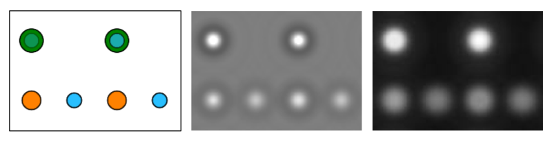
[Left: projected SrTiO3 structure, Center: amplitude, and Right: phase of the wavefunction of a 2.8 nm thick crystal (20 slices). In the structure projection Sr atoms are displayed in green color, Ti in orange, and Oxygen in blue. Amplitude and phase of the wavefunction are displayed in a grayscale over the range from 0.0 (black) to 2.0 (white).]
The images above show the projected atomic structure on the left side, with Sr atoms in green color, Ti atoms in orange, and O atoms in blue. Amplitude and phase of the wavefunction after 20 slices (2.8 nm object thickness) of the multislice calculation are displayed in the center and right respectively. The strongest peaks in amplitude and phase appear at the positions of the SrO columns, peaks of intermediate strength at Ti columns, and the weakest peaks appear at the positions of pure oxygen columns.
Image calculations with WAVIMG
In the electron microscope we record the absolute square of a wavefunction which has been magnified by passing through a system of lenses, the so-called image-plane wavefunction. The image-plane wavefunction is additionally modulated due to aberrations, and the imaging process itself is affected by partial losses of coherence and further incoherent phenomena, which all essentially lead to a reduction of the image contrast.
The program WAVIMG can be used to calculate high-resolution TEM images from exit-plane wavefunctions. Calculations with WAVIMG are again controlled by a text parameter file similar to that used for MSA before. The structure and content of this parameter file is described in detail in the online documentation of the program WAVIMG.
We will store the parameter file for WAVIMG again in the sub-folder 'prm' of our working directory. In the course of this example, we will use three different parameter files for image simulations with WAVIMG, (1) for the calculation of a single image of SrTiO3 [110], (2) for the calculation of a focal series, and (3) for the calculation of focus-over-thickness map.
(1) Single image calculation
The text block below shows the content of the first parameter file, which
you can copy from here into your text editor, e.g. notepad.exe.
'wav\STO_110_300_sl020.wav' ! wave function file name
128, 90 ! [pix, pix] wave function samples
0.004315, 0.004339 ! [nm/pix] wave function sampling rates
300. ! [keV] primary electron energy
0 ! image output type
'img\STO_110_300.dat' ! image output file name
64, 45 ! [pix, pix] image samples
0, 1., 1., 0. ! [switch, mean, cts/el., noise] image data type
1 ! [switch] use image frame
0.008690 ! [nm/pix] image sampling rate
0.0, 0.0 ! [pix, pix] image offset in wave frame
0.0 ! [deg] image frame rotation
1 ! coherence model switch (1 ... 5)
1, 3.5 ! [switch, nm] focus-spread
1, 0.5 ! [switch, mrad] semi-convergence
1, 1., 'MTF-US2k-300.mtf' ! [switch, scale, file name] detector MTF
1, 0.02, 0.02, 0. ! [model, nm, nm, deg] vibration envelope
2 ! number of image aberrations
1, 4.2, 0. ! [ID, nm, nm] aberration coefficients ID=1: C1
5, -15000., 0. ! [ID, nm, nm] aberration coefficients ID=5: C3
250. ! [mrad] image objective aperture
0., 0. ! [mrad] image objective aperture center
0 ! number of parameter loops
Please, store the parameter file in the sub-folder 'prm' using the file name 'wavimg-1.prm'. Alternatively, you may download the parameter file. The downloaded archive contains all three parameter files of this example. Please, put all three files into the 'prm' sub-folder.
Before starting the program, please make sure that all data is present as specified in the parameter file. This means the input wave function files and the MTF file 'MTF-US2k-300.mtf'. In the way how the parameter file is written above, WAVIMG expects the MTF file to be in the directory from where you call the program, i.e. the working directory. You may also use a full path and file name to link to MTF data somewhere else on your computer storage.
With all parameters set up properly, you can now run WAVIMG by calling
wavimg -prm prm\wavimg-1.prm
which will output a raw binary data file in the sub-folder 'img' with the file name 'STO_110_300.dat'. The file contains a list of intensity values, which are the image intensities arranged in an array of 64 x 45 pixels as specified in line 7 of the parameter file. The intensity values are stored as 32-bit floating point data.
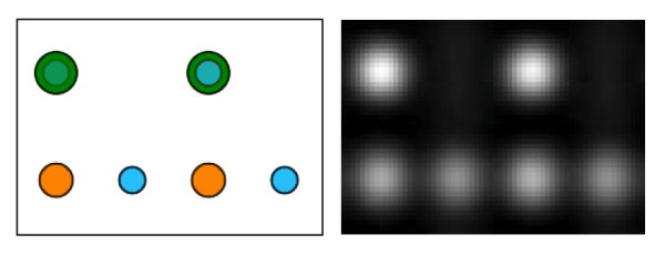
Left: projected SrTiO3 structure, Right: calculated HR-TEM image of a 2.8 nm thick crystal (20 slices). In the structure projection Sr atoms are displayed in green color, Ti in orange, and Oxygen in blue. The gray scale image covers the intensity range from 0.75 (black) to 1.85 (white) where the incident beam intensity is 1.0.
The images above show the atomic structure of SrTiO3 on the left side, with Sr atoms in green color, Ti atoms in orange, and O atoms in blue. The calculated image of a 2.8 nm thick SrTiO3 crystal is displayed on the right. The strongest intensity peaks appear at the positions of the SrO columns, peaks of intermediate strength at Ti columns, and the weakest peaks appear at the positions of pure oxygen columns.
2) Focal series calculation
In the second part of this TEM simulation example, we will calculate a focal series of SrTiO3 [110] again with 2.8 nm object thickness in slightly larger images. For this purpose we modify the parameter file in a few lines and store the changed file in the sub-folder 'prm' under the file name 'wavimg-2.prm'.
In order to increase the size of the image by 2 x 3 of the previous size to images of 128 x 135 pixels, we change the numbers in line 7 of the parameter file respectively, reading now
...
128, 135 ! [pix, pix] image samples
...
The automatic calculation of a focal series is set up via the loop functions
of WAVIMG. We need here one loop over an aberration coefficient, the defocus.
To set up the focus loop, please change the number in line 23 from
0 to 1, which indicates that one parameter loop
should be performed. Further append additional lines below line 23 just as listed
in the text block below!
...
1 ! number of parameter loops (line 23)
1 ! loop parameter class, 1 = aberration
1 ! loop parameter index, 1 = defocus
1 ! loop variation form, 1 = ramp
-10.0, 10.0, 41 ! [nm, nm, number] loop range and samples
'unused' ! loop string
Using this parameter file in the call to WAVIMG
wavimg -prm prm\wavimg-2.prm
a series of 41 raw binary data files is created in the sub-folder 'img' with the file names 'STO_110_300_001.dat', 'STO_110_300_002.dat', ... , 'STO_110_300_041.dat'. The files contain images of the 2.8 nm thick SrTiO3 crystal in [110] projection with image defoci changing between -10 nm and +10 nm in steps of 0.5 nm. The focal series is displayed below as animation of grayscale images.
Focal series of SrTiO3 [110] showing 2 x 3 of the previous structure units. The image defocus is indicated in the annotation.
3) Calculation of a focus-over-thickness map
Since both, defocus and object thickness have a significant effect on the image intensity distribution, one often calculates a focus-over-thickness map in order to roughly estimate the values of these two parameters for an experimental image by visual comparison. WAVIMG provides a function for the creation of 2D parameter variation maps, which will be demonstrated in the following. For this purpose we modify the WAVIMG parameter file of the previous steps in a few lines and store the changed file in the sub-folder 'prm' under the file name 'wavimg-3.prm'.
The first change is made already in line 1, where we tell WAVIMG, which exit-plane wavefunction is used for the image calculation. For a variation of the object thickness, we actually need different wavefunctions as input. A series of wavefunctions with increasing object thickness has been calculated by MSA in this example. The wave function files differ in their file name by a numerical index starting from '001' up to '040', indicating the number of object structure slices used for the calculation of the respective wavefunction. This means the wavefunction 'wav\STO_110_300_sl027.wav' was extracted from the multislice calculation after the application of the object transmission function in slice number 27, corresponding to an object thickness of 3.7 nm. In order to allow WAVIMG to load any of these exit-plane waves, we change the string in line 1 to the common parts of the 40 wavefunction files names, which is 'wav\STO_110_300_sl.wav':
'wav\STO_110_300_sl.wav' ! common wavefunction file name (line 1)
...
As a second step we tell WAVIMG to calculate a 2d parameter variation map by changing the image output type in line 5 and change the output file name in line 6 to prevent overwriting of previous images:
...
6 ! image output type 6 = map (line 5)
'img\STO_110_300_map.dat' ! image output file name (line 6)
...
Accordingly the map image will be saved to the file 'img\STO_110_300_map.dat'.
We will compose the map of focal changes in a first loop over a range from 0.5 nm up to 10.0 nm defocus in 20 steps, and over wavefunctions of objects with 2, 4, 6, ..., up to 40 slices in a second loop. We choose now th size of the map such that a [110] unit cell is displayed for each combination of defocus and thickness. As a unit cell covers 64 x 45 pixels when using the same sampling rate as in the previous calculations, we need an image of 1280 x 900 pixels to cover the complete variation range. Accordingly the output image size is changed in line 7 of the parameter file:
...
1280, 900 ! [pix, pix] image samples (line 7)
...
Finally we modify the whole loop section starting from line 23 in the following way:
...
2 ! number of parameter loops (line 23)
1 ! loop parameter class, 1 = aberration
1 ! loop parameter index, 1 = defocus
1 ! loop variation form, 1 = ramp
0.5, 10.0, 20 ! [nm, nm, number] loop range and samples
'unsused' ! loop string
3 ! loop parameter class, 3 = input wave files
1 ! loop parameter index, ignored
1 ! loop variation form, 1 = ramp
2.0, 40.0, 20 ! [ID, ID, number] loop range and samples
'_sl' ! loop string, prefix before wave number
The loop section contains now 2 loops as set in line 23. The first loop is very similar to the loop of the focal series simulation, except for a reduced focal range. The second loop is a loop over input wavefunctions. The wavefunctions are identified by their file name as given in line 1 plus a sub-string containing a three-digit number, which is inserted directly after the sub-string '_sl'. The inserted sub-string is changing with each step of the loop, where the first number is 2 and the respective sub-string is '002', and where the last number is 40 and the respective sub-string is '040'. The second loop has 20 samples, such that the thickness variation is performed in steps of 2 slices.
Using the third parameter file in the call to WAVIMG will initiate longer
calculation, since an image is produced for each step of the nested loops.
As we are not interested in these individual images, but in the total map
image alone, we apply the option /nli to prevent WAVIMG from
saving the individual loop images:
wavimg -prm prm\wavimg-3.prm /nli
The resulting image 'img\STO_110_300_map.dat' is a raw binary data file containing the map image in 1280 x 900 32-bit floating point intensity values. The map image is displayed below with annotations indicating the scale of the horizontal defocus and the vertical thickness axis.
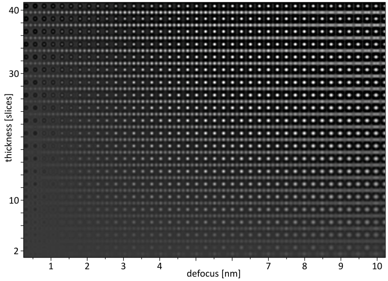
HR-TEM focus over thickness map of SrTiO3 [110].
Last update: Feb 6, 2024 contact disclaimer(de)